Rni.helsinki.fi

The Binomial Distribution: Logistic Regression A common type of data that is encountered is when there is a binary outcome. Examples includewhether a subject survives or dies from some treatment. Statisticians usually talk about theoutcomes (Yi) from the ith trial (i=1,.,n) as being "success" (Yi=1) and "failure" (Yi=0). These areassumed to be stochastic, so there is a probability associated with each one: Usually we have a set of p covariates, xij (j=1,.,p) measured on each trial, and the statisticalproblem is to determine which covariates affects the probability of a success. This leads on to theidea that each observation is a Bernoulli trial.
If the covariates are made up of a discrete number of classes, then we can present the data in twoways: Subject
Covariate, x
Response, Y
Covariate, x
Class Size, m
Response, Y
This second way of writing the table is more efficient, especially when the number of trials (n)increases. The classic situation where this sort of data is seen in in contingency tables. For example, for thedata above, the 2x3 contingency table would look like this: For our present purposes, interest focusses on how the response probabilities are arranged over thedifferent values of x, but not the distribution of the x's themselves - methods for dealing with thelatter problem will be discussed later. We therefore consider the marginal totals (the m's) fixed.
The natural model for this data is to assume that each trial is a Bernoulli trial. If we assume that thetrials are independent, then for trials with the same covariates, the distribution of successes in the mtrials is a binomial distribution: P Y = y∣m=my1−m−y .
The usual notation for this is Y ~ Bin(m, π). The Bernoulli distribution is a special case, with m=1.
l ∣y= y log m− ylog 1− The natural parameter is therefore b =log  . Here the data is re-coded as the proportion of successes (so that E(y/m)=π). We can see that the dispersion parameter is 1/m. Any function that maps from [-∞,+∞] to [0,1] will work as a link function. However, there are onlythree link functions that commonly used: 1. Logit link, g ==log  This is the canonical link function. This has the range [-∞,+∞] (because 0≤π≤1, so and hence can be additive. The inverse link function is g 1 x = e  .
The logit link has a fairly simple interpretation, as the log-odds. 1− is the odds of a success (i.e. for every failure there are 1− successes). The logit is simply the log of this. The interpretation of the logit can be seen from looking at a 2x2 contingency table like this: The empirical odds for y at x=0 is simply b/a. Similarly the empirical odds at x=1 is d/c. If these were equal, i.e. if b/a = d/c, then / d =1 . This is called the odds ratio. If the odds ration is different from 1 represents then there is an effect of x on the probability of a success (i.e. y=1). Thisempirical ratio is easy to calculate, and the log of the ratio is just ln b - ln a + ln c - ln d, i.e. it islinear on this scale and a value of zero represents no effect. There is one useful property that arises out of the logit transformation. In medical studies, there aretwo approaches to studying factors influencing disease risk. One is a prospective study, where agroup of exposed subject and non-exposed subject are chosen, and then followed to see theproportion in each group that succumb to the disease. The numbers of subjects in each group aretherefore fixed, and the numbers with the disease are random.
The second type of study is a retrospective study. Here, diseased and disease free individuals arechosen (from hospital records, for example), and the numbers exposed and not exposed to the factorare counted. The numbers with or without the disease are fixed, and the numbers exposed arerandom. In both cases the data will be in a contingency table form, as in the table above. Consider theprospective study first. the logits for the two groups are log(a/b) and log(c/d). The difference isthus =loga/b−logc/d =loga−logb−logclogd  .
For the retrospective study, we can estimate the difference in the proportion of individuals in eachdisease group who were exposed to the factor. This is: log a /c−log b /d =log a−log c−log blog d = .
In other words, the same effect is estimated in both cases. In practice, a retrospective study will bemore efficient, as diseases are often rare, so the sample sizes needed will be smaller. This propertycan be generalised to more complex analyses, and does not hold for the other link functions that arecommonly used.
2. Probit linkThis is the inverse Normal distribution: where Φ(⋅) is the cumulative Normal distribution function, i.e.
This link was developed from the analysis of dose-response curves. These are often estimated bydividing animals into groups of, say, 20, and exposing each group to a different dose (i.e.
concentration) of a poison. The higher the dose, the higher the proportion of animals that will die.
Typically, the doses are equally spaced on the log-scale. The model then assumes that theprobability of an individual dying is where α and β are parameters to be estimated. Typically, the main parameter of interest is the doseat which half of the animals die - the LD50 or ED50 dose (LD="Lethal Dose", ED="effective dose",which sounds nicer and so has not caught on). This dose is at -α/β. Another area where this model is used is in quantitative genetics, where it is used to modelthreshold traits. An example of this is hexadactyly in pigs, where most pigs have 5 toes, but somehave 6. This is controlled by many genes, each with a small effect (say, the concentration of achemical). Over a population, their effect will follow a Normal distribution (by Central LimitTheorem). The theory is that there is a threshold that if exceeded, means that the pig will have 6toes. If there is environmental variation as well, then this may work on the same scale. Hence, theobserved effect will follow a Normal distribution (with some mean and variance), and the probability that the threshold is exceeded is the inverse Normal c.d.f. (or rather 1 minus that).
Both the logit and probit link functions are symmetrical about π=0.5, but this is not a necessity. Anasymmetric alternative is the complementary log-log link, commonly abbreviated to cloglog.
Historically, this was the first link function to be developed (in 1922!). The function is g =log −log 1− The motivation comes from dilution assays. These are commonly used in microbiology to estimatethe concentration of a bacterium in a culture. The culture is repeatedly diluted, for simplicity wecan assume that the dilution is by half each time. If there are any bacteria in a dilution, they will beseen (they grow, and make the culture cloudy). From this pattern, the concentration of bacteria canbe estimated.
If the initial concentration is ρ0, then after x dilutions the concentration is ρ0/2x. If each culture has avolume v, then the expected number of bacteria in each culture is vρ0/2x. If we assume good mixing,then the actual number will follow a Poisson distribution. Hence, the probability that the culture isinfected is πx = 1 - exp(-ρxv). Therefore, at dilution x, log −log 1− =log vlog  =log vlog  − x log 2 The general motivation for the cloglog link is that in each trial, we have a Poisson process, and ifthere are no events then we have a failure.
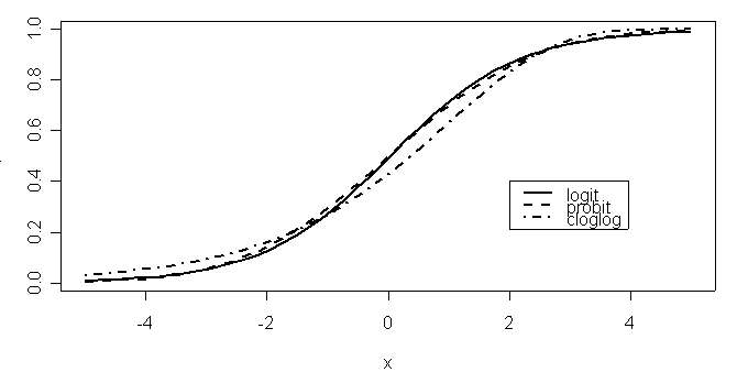
The different link functions are different relationships between η and π. These are plotted below.
All three are from models fitted to the same data. The logit and probit curves are very similar, andare symmetrical about x=0. For data in the middle of the range (about 0.2<π<0.8), they areindistinguishable, and indeed are close to being straight lines. The cloglog curve is asymmetrical,with a longer tail at the lower end.
The (log-) likelihood for a binomial distribution, with a general link function, g() is l ∣y=∑  y g  m log1−  ignoring the ∑ logmi term. For a logit link, we have g = =log i =∑ x  , l ∣y=∑ ∑ y x  ∑ m log An important point here is that the log likelihood only depends on the βj's through the linear . These p combinations are sufficient statistics for the βj's. This property is a result of the logit link being the canonical link function.
The parameter estimates can be found by firstly differentiating l(πι|y) w.r.t. βj, which (from lecture2) is the score, Uj: As the distribution is binomial, we know that E(y (note to me: ∂  /∂  =m ∂  /∂  =∑  y −m   x or, in matrix form, XT(Y-µ). The likelihood
equations then amount to equating the sufficient statistic XTY to its expectation, as a function of β.
In practice the calculations are carried out by computer using an iterative scheme. For all three linkfunctions here, the algorithm will converge unless one of the  's is infinite, which is equivalentto having a fitted probability of 0 or 1. In practice, this normally means that you get a warning fromthe computer. The estimated deviances are usually reasonable, as the fitted values are accurate (asthey are close to 1 or 0), but the estimates are usually fixed at a large (or small!) value, and thestandard errors may well be wrong. The deviance is just -2l, and we have ∣x=∑ {y log  m − y log1−  }
(just re-writing the likelihood above). The maximum is at the points   = y /m , so the residual D  y∣ 
∣y−2l  ∣y
2∑ {y log yim −y logmi i} This behaves like a residual sum of squares in an ANOVA. The difference between two deviancesis approximately a chi-squared distribution. Asymptotically, the residual deviance is also a chi-squared distribution. However, the asymptotics may not always work correctly – there will be anexample later.
Once we get beyond the theory, the actual analyses look similar to a linear model. We can thereforeuse the same techniques to model building and comparison as with a linear model.
For example, here is some data from a study of the effectiveness of drugs to prevent post-operativenausea (i.e. people throwing up after having an operation).
Drug
No. of patients
Incidences of nausea
First, we can see if the drugs make any difference: we compare the null model (i.e. with only aconstant) to the model with Drug as a factor. The code is from R (but I have removed some of theoutput): > glm1 <- glm(NN~Drug, family=binomial()) So, there is an effect in there. The next thing to do is to find out where it is. We can get theparameter estimates: Estimate Std. Error z value Pr(>|z|) (Intercept) 0.30538 0.15752 1.939 0.0525 . chlorpromazine -0.95931 0.23247 -4.127 3.68e-05 *** dimenhydrinate 0.14935 0.27266 0.548 0.5839 pentabarbital100 -0.21577 0.29092 -0.742 0.4583 pentabarbital150 -0.09566 0.29184 -0.328 0.7431 Signif. codes: 0 `***' 0.001 `**' 0.01 `*' 0.05 `.' 0.1 ` ' 1 The estimates are calculated as contrasts from the first level of the factor. Conveniently, this is theplacebo. We can therefore see that Chlorpromazine gives a lower probability of nausea (which isgood), but the others do not seem to make much of a difference.
We can get a more visual summary from a graph: The error bars are 1 standard error. We can now clearly see that chlorpromazine is the only drugthat has an effect.
How strong is the effect? The point estimate is the log odds, and is -0.96, so the odds are e-0.96 =0.38. In other words, nausea is 2.6 times (=1/0.38) less likely with the drug.

Source: http://www.rni.helsinki.fi/~boh/Teaching/GLMs/glmsl6.pdf